【特征匹配】SIFT原理与C源代码剖析(2)

构建高斯金字塔（octave = 5, intervals+3=6）：

所有空间尺度为：

在极值比较的过程中，每一组图像的首末两层是无法进行极值比较的，为了满足尺度变化的连续性（下面有详解），我们在每一组图像的顶层继续用高斯模糊生成了 3 幅图像，高斯金字塔有每组s+3层图像。在计算视觉领域，尺度空间被象征性的表述为一个图像金字塔，其中，输入图像函数反复与高斯函数的核卷积并反复对其进行二次抽样，这种方法主要用于sift算法的实现，但每层图像依赖于前一层图像，并且图像需要重设尺寸，因此，这种计算方法运算量较大，而surf算法申请增加图像核的尺寸，这也是sift算法与surf算法在使用金字塔原理方面的不同。高斯函数的方差当然还是与这个特征点所在的图像层的尺度有关，就是。

高斯金字塔是通过高斯平滑和亚采样获得一些列下采样图像，也就是说第k层高斯金字塔通过平滑、亚采样就可以获得k+1层高斯图像，高斯金字塔包含了一系列低通滤波器，其截至频率从上一层到下一层是以因子2逐渐增加，所以高斯金字塔可以跨越很大的频率范围。在极值比较的过程中，每一组图像的首末两层是无法进行极值比较的，为了满足尺度变化的连续性（下面有详解），我们在每一组图像的顶层继续用高斯模糊生成了 3 幅图像，高斯金字塔有每组s+3层图像。作为特征提取的一个前提运算，输入图像一般通过高斯模糊核在尺度空间中被平滑，此后通过局部导数运算来计算图像的一个或多个特征。

洗 选 后 煤 的 灰 分 大 幅 度 下 降 ,浮 煤 一 般 均 不 大 于 10%,为 特 低 灰分 煤 ( sla) ,仅 7 煤 有 5 个 层 点 样 ( 占 5%), 12-1 煤 有 2 个 层点 样 ( 占 2%) ,12-2 煤 有 6 个 层 点 样 ( 占 5%), 13 煤 有 3 个 层点 样( 占 3%),为 低 灰 分 煤( la)。图像复原要求对图像降质的原因有一定的了解，一般讲应根据降质过程建立“降质模型”，再采用某种滤波方法，恢复或重建原来的图像。待投影实际图像时，只须将各象元的灰级数，以及该象元的基准电压按一定关系就可算出需加在该象元上的电压值了。

但在原图上看。形成了所有的空间尺度。

☆3.每组（octave）有S+3层图像，是因为在DOG尺度空间上寻找极值点的方法是在一个立方体内进行，即上下层比較。所以不在DOG空间的第一层与最后一层寻找，即DOG须要S+2层图像，因为DOG尺度空间是由高斯金字塔相邻图像相减得到，即每组须要S+3层图像。

/*
  Builds Gaussian scale space pyramid from an image
  @param base base image of the pyramid
  @param octvs number of octaves of scale space
  @param intvls number of intervals per octave
  @param sigma amount of Gaussian smoothing per octave
  @return Returns a Gaussian scale space pyramid as an octvs x (intvls + 3)
    array 
	
给定组数(octave)和层数(intvls)。以及初始平滑系数sigma,构建高斯金字塔
返回的每组中层数为intvls+3
*/
static IplImage*** build_gauss_pyr( IplImage* base, int octvs,
			     int intvls, double sigma )
{
  IplImage*** gauss_pyr;
  const int _intvls = intvls;             // lowe 採用了每组层数(intvls)为 3
 // double  sig_total, sig_prev;
	 double  k;
  int i, o;
  double *sig = (double *)malloc(sizeof(int)*(_intvls+3));  //存储每组的高斯平滑因子，每组相应的平滑因子都同样
  gauss_pyr = calloc( octvs, sizeof( IplImage** ) );              
  for( i = 0; i < octvs; i++ )
    gauss_pyr[i] = calloc( intvls + 3, sizeof( IplImage *) );
  /*
    precompute Gaussian sigmas using the following formula:
    \sigma_{total}^2 = \sigma_{i}^2 + \sigma_{i-1}^2
    sig[i] is the incremental sigma value needed to compute 
    the actual sigma of level i. Keeping track of incremental
    sigmas vs. total sigmas keeps the gaussian kernel small.
  */
  k = pow( 2.0, 1.0 / intvls );                 // k = 2^(1/S)
  sig[0] = sigma;
  sig[1] = sigma * sqrt( k*k- 1 );
  for (i = 2; i < intvls + 3; i++)
      sig[i] = sig[i-1] * k;                       //每组相应的平滑因子为 σ ,  sqrt(k^2 -1)* σ, sqrt(k^2 -1)* kσ , ...
  for( o = 0; o < octvs; o++ )
    for( i = 0; i < intvls + 3; i++ )
      {
	if( o == 0  &&  i == 0 )
	  gauss_pyr[o][i] = cvCloneImage(base);                       //第一组。第一层为原图
	/* base of new octvave is halved image from end of previous octave */
	else if( i == 0 )
	  gauss_pyr[o][i] = downsample( gauss_pyr[o-1][intvls] );  //第一层图像由上一层倒数第三张隔点採样得到
	  
	/* blur the current octave's last image to create the next one */
	else
	  {
	    gauss_pyr[o][i] = cvCreateImage( cvGetSize(gauss_pyr[o][i-1]),
					     IPL_DEPTH_32F, 1 );
	    cvSmooth( gauss_pyr[o][i-1], gauss_pyr[o][i],
		      CV_GAUSSIAN, 0, 0, sig[i], sig[i] );                       //高斯平滑
	  }
      }
     
   
  return gauss_pyr;
}

Lindeberg发现高斯差分函数（DifferenceofGaussian。简称DOG算子）与尺度归一化的高斯拉普拉斯函数很近似，且

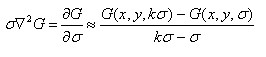
差分近似：

lowe建议採用相邻尺度的图像相减来获得高斯差分图像D(x,y,σ)来近似LOG来进行极值检測。

D(x,y,σ) = G(x,y,kσ)*I(x,y)-G(x,y,σ)*I(x,y)

=L(x,y,kσ) - L(x,y,σ)

对高斯金字塔的每组内相邻图像相减。形成DOG尺度空间，这时DOG中每组有S+2层图像

static IplImage*** build_dog_pyr( IplImage*** gauss_pyr, int octvs, int intvls )
{
  IplImage*** dog_pyr;
  int i, o;
  dog_pyr = calloc( octvs, sizeof( IplImage** ) );
  for( i = 0; i < octvs; i++ )
    dog_pyr[i] = calloc( intvls + 2, sizeof(IplImage*) );
  for( o = 0; o < octvs; o++ )
    for( i = 0; i < intvls + 2; i++ )
      {
	dog_pyr[o][i] = cvCreateImage( cvGetSize(gauss_pyr[o][i]),
				       IPL_DEPTH_32F, 1 );
	cvSub( gauss_pyr[o][i+1], gauss_pyr[o][i], dog_pyr[o][i], NULL );   //相邻两层图像相减，结果放在dog_pyr数组内
      }
  return dog_pyr;
}

在DOG尺度空间上，首先寻找极值点，插值处理，找到准确的极值点坐标，再排除不稳定的特征点（边界点）

/*
  Detects features at extrema in DoG scale space.  Bad features are discarded
  based on contrast and ratio of principal curvatures.
  @return Returns an array of detected features whose scales, orientations,
    and descriptors are yet to be determined.
*/
static CvSeq* scale_space_extrema( IplImage*** dog_pyr, int octvs, int intvls,
				   double contr_thr, int curv_thr,
				   CvMemStorage* storage )
{
  CvSeq* features;
  double prelim_contr_thr = 0.5 * contr_thr / intvls; //极值比較前的阈值处理
  struct feature* feat;
  struct detection_data* ddata;
  int o, i, r, c;
  features = cvCreateSeq( 0, sizeof(CvSeq), sizeof(struct feature), storage );
  for( o = 0; o < octvs; o++ )                     //对DOG尺度空间上，遍历从第二层图像開始到倒数第二层图像上。每一个像素点
    for( i = 1; i <= intvls; i++ )
      for(r = SIFT_IMG_BORDER; r < dog_pyr[o][0]->height-SIFT_IMG_BORDER; r++)        
	for(c = SIFT_IMG_BORDER; c < dog_pyr[o][0]->width-SIFT_IMG_BORDER; c++)
	  /* perform preliminary check on contrast */
	  if( ABS( pixval32f( dog_pyr[o][i], r, c ) ) > prelim_contr_thr )    // 排除像素值小于阈值prelim_contr_thr的点，提高稳定性
	    if( is_extremum( dog_pyr, o, i, r, c ) )             //与周围26个像素值比較，是否极大值或者极小值点
	      {
		feat = interp_extremum(dog_pyr, o, i, r, c, intvls, contr_thr); //插值处理，找到准确的特征点坐标
		if( feat )
		  {
		    ddata = feat_detection_data( feat );
		    if( ! is_too_edge_like( dog_pyr[ddata->octv][ddata->intvl],   //依据Hessian矩阵 推断是否为边缘上的点
					    ddata->r, ddata->c, curv_thr ) )
		      {
			cvSeqPush( features, feat );          //是特征点进入特征点序列
		      }
		    else
		      free( ddata );
		    free( feat );
		  }
	      }
  
  return features;
}